The LDA notebook
Using the LDA topic modeling notebook
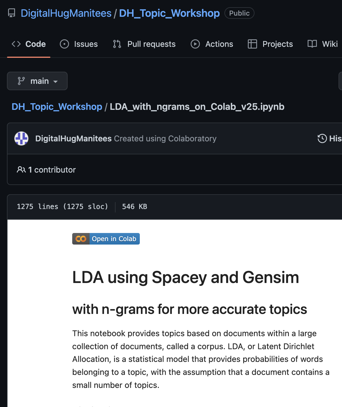
You can find the LDA notebook here on GitHub.
About Google Colab
Google Colab is a Jupyter Notebook that runs on Google’s servers, allowing you to run Python code on data calculated and stored on cloud servers. This is great for large, computationally heavy projects where processing can be increased easily with a few lines of code. Unlike Jupyter notebooks run locally on your computer, the Colab environment is independent of your locally installed environments, meaning that you are less likely to run into conflicts. The downside to the Google Colab environment is that any information created in Colab is erased when you close the browser, unless you save it somewhere, like GitHub or locally on your computer.
Process guide for the LDA topic modeling notebook
Step 1:
There are two ways to open the LDA notebook:
open through Github - you will use this process the first time opening the notebooks. Look for the ‘open in Colab’ button.
- Save a copy of this notebook to your Google Drive. All changes will be saved to your own copy.
Open through Colab - You can use this process if you have previously saved it to your Google Drive.
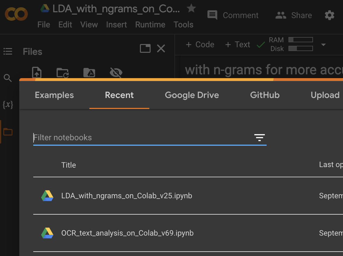
In Colab, go to File>Open. This will open a dialog box.
At the top tabs of the dialog box, select Google Drive - you should see your previously saved copy.
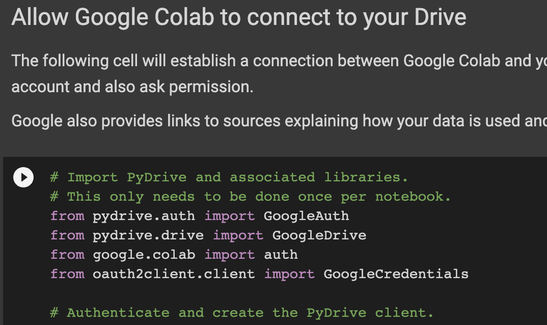
Run the first cell - this will connect to your Google Drive. A dialog box will open and ask you to select your Google account and ask for your permission to connect to your Google Drive.
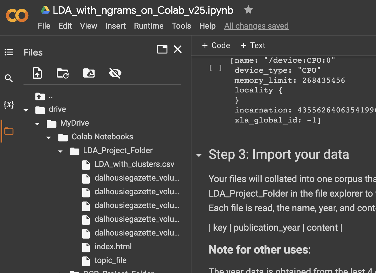
It will also create a new directory in your Google Drive for all of the files needed for this project. You should see something like this indicating your new working directory.
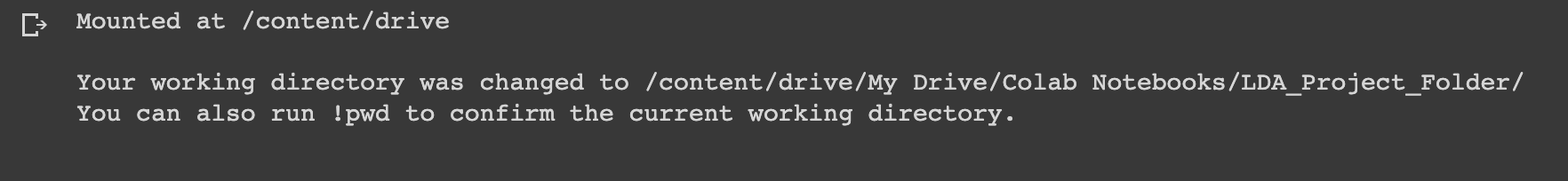
Run the cell that connects Colab to your drive. This gives permissions for information to be shared between the two and provides a safe place to store the results of your analysis.
Your working directory is now set as folders on your Google Drive. All files saved here will be safe and not deleted when you close the notebook.
Step 2:
Install the libraries and dependencies needed for this notebook.
This cell also installs the spaCy model that is used to train the algorithm. There are different models as well as a wide range of language support. You can read more about them here.
Step 3:
Import your data. Remember all those text files you created using the OCR notebook? Before running the cell in Step 3, move all your .txt files to the working directory in your Google Drive. You can drag them from your file manager (Finder in Mac, Explorer in Win) directly into the Colab file manager on the left.
Step 4:
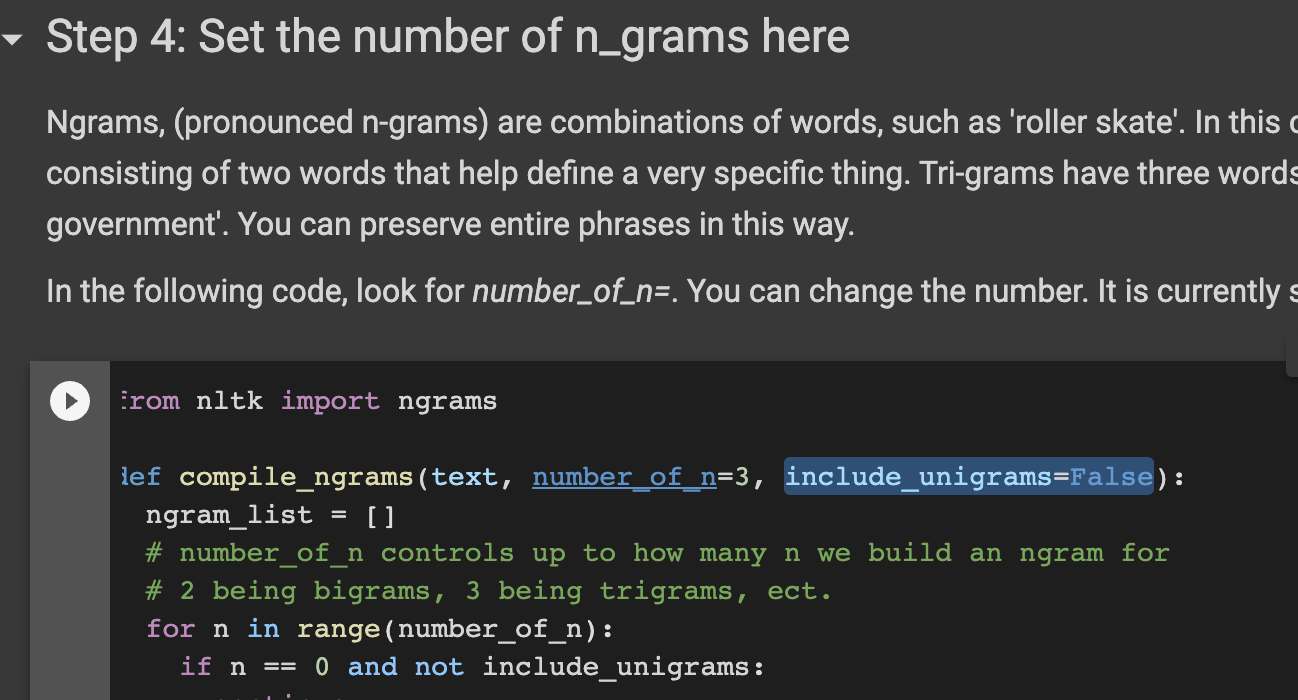
Set the number of n-grams. These are word combinations that are particular to your text. As an example, 2-grams, or bigrams, are word combinations like ‘Dalhousie University’ or ‘roller skate’. If they are separated, then contextual meaning can be lost. Whole phrases can be maintained this way, though specific phrases can be preserived at a later step.
You can adjust the n-grams at the code marked number_of_n=3. In this case, word combinations up to trigrams are preserved.
Allowing unigrams (singular words) can also be permitted. However, these can dominate due to their increased frequency and should be tried to see if if improves your results. Look for the code include_unigrams=False and change False to True if you wish to include unigrams.
Step 5:
Step 5 cleans the data by removing unneccesary words, punctuations, and symbols. You can also preserve certain phrases or words if they are important to you. Look for the code author_assigned_keywords =` and type each phrase or word you want inside double quotes, separating each with commas.
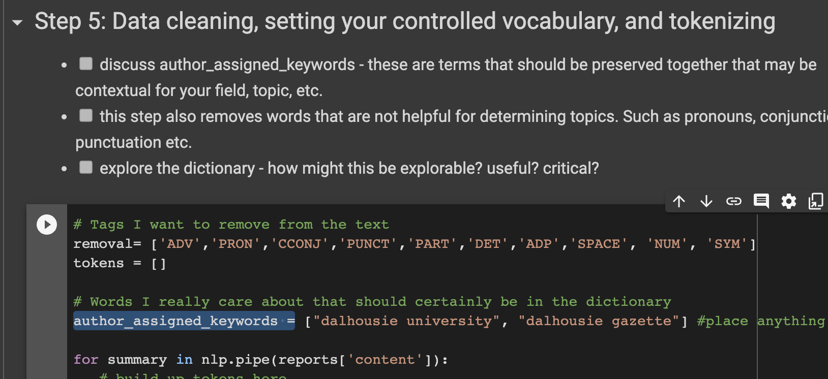
Completing step 5 will have created tokens and placed each documents tokens in a table along with the file name, document year, and content for further analysis.
Step 6:
This cell runs several processes we should be aware of.
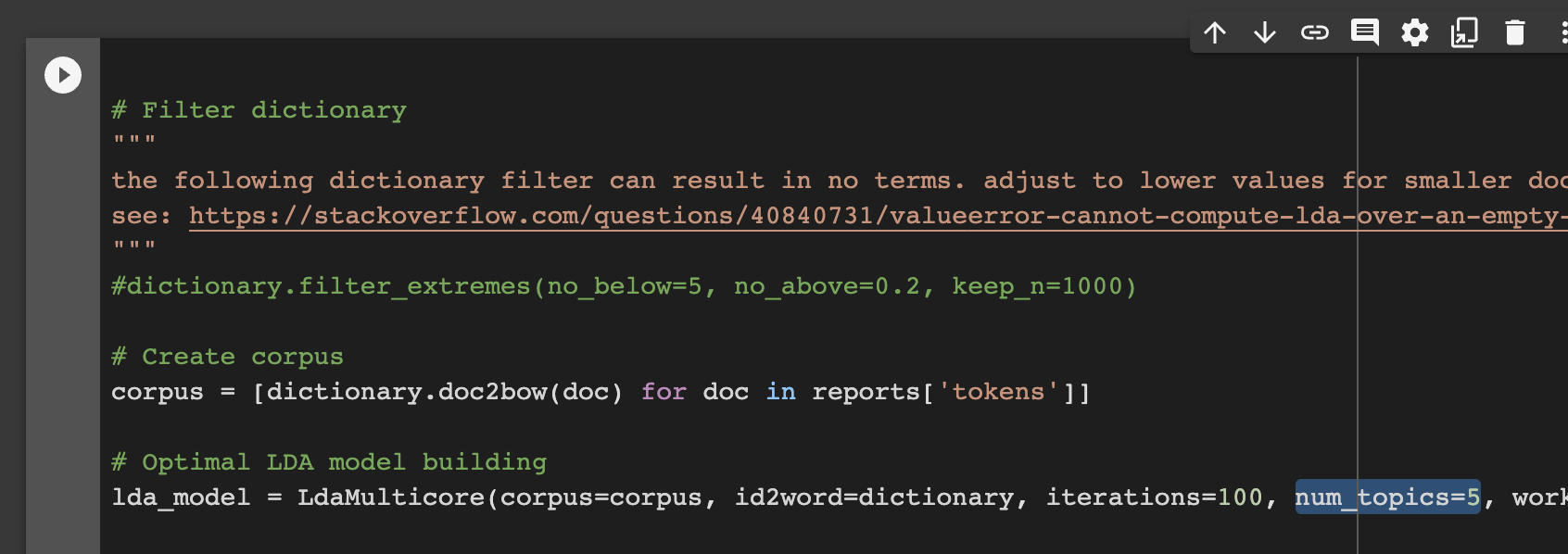
It applies a filter against the dictionary to reduce extremes. With small corpora, we need to turn this off as you can see with the
#before the line#dictionary.filter_extremes(no_below=5, no_above=0.2, keep_n=1000). If you are using a large corpus, then remove the#to make this line functional again.It runs the LDA analysis with settings that can be adjusted, such as
num_topics=5. In this case, 5 topics has already been specified. You can increase or decrease as you need.
It creates the pyLDAvis interactive webpage or results. This will be deposited in your working directory.
Step 7:
The final step in our process creates additional output from the analysis that may be useful for information retrieval or other analysis.
The number of topics are printed along with their score.
The topics and top 10 words/phrases are printed. You can cut and paste these into Excel or a table in a document for reporting.
A Pandas table is created with the cluster and score next to each document, (since this was a document level clustering analysis). The table is exported as a .csv and saved in your working directory.
That’s it!
That is the final step in the analysis! You may want to move the filles you used for the analysis and the results into another folder if you’d like to analyze another batch. Simply move them, and put more .txt files into the working directory and you can repeat the notebook from Step 3.
Your examples should look something like this example from a project that investigated ‘teaching effectiveness’ across a corpus of articles.
Optional:
There is a testing option for evaluating the number of topics. This works best on large corpora compared with small ones. The coherence scores were a conventional way to evaluate topic analysis, but it is beginning to fall out of favor with newer methods.
You can read more about coherence here and here (though this is an ad-heavy website, but the explanation is helpful).
The graph is read as coherence closer to 0 is better.
Future improvements & applications
improve the pyLDAvis to show file names as a mouseover or separate table.
explain more of the tuning parameters to LDA.
Evaluate unsupervised models versus trained models